| Filename |
Contents |
| run_models.py |
Script that runs tests with two ASCAD
models and the simpler models |
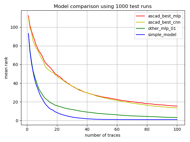
| model_comparison.png |
Graphics output created with: python3
run_models.py 1000 100 |
| AES_Sbox.py |
AES S-Box table used by run_models.py |
| ascad_best_mlp.py |
Wrapper for ASCAD "best MLP" model |
| ascad_best_cnn.py |
Wrapper for ASCAD "best CNN" model |
| simple_model.py |
The simple model presented here |
| simple_model.bin |
Numpy arrays used in the simple model |
| mk_simple_model.py |
The script that was used to create simple_model.bin |
| other_mlp_01.py |
Wrapper for another MLP model |
| other_mlp_01.h5 |
Saved parameters for that other MLP |
| train_other_mlp_01.py |
The script that was used to create
other_mlp_01.h5 (will overwrite when re-run) |
import numpy as npAssembling a pile of numbers as in simple_model.bin is left as an exercise to the reader (it is less than 48 KByte), or you may use the script mk_simple_model.py supplied in the tarball to learn how it was done.
f = open('simple_model.bin', 'rb')
pr = np.fromfile(f, dtype=np.float32, count=10*700).reshape(700,10)
mR = np.fromfile(f, dtype=np.float32, count=10*256).reshape(256,10)
mX = np.fromfile(f, dtype=np.float32, count=10*256).reshape(256,10)
f.close()
S = np.tile(np.arange(0x100, dtype = np.uint8).reshape(1,256), (256,1))
R = np.tile(np.arange(0x100, dtype = np.uint8).reshape(256,1), (1,256))
X = S ^ R
m = mR[R,:] + mX[X,:]
def predict(batch):
upr = batch.dot(pr).reshape(-1,1,1,10)
return np.exp(-.5 * ((upr - m) ** 2).sum(3)).sum(1)
m = Sequential([A non-trainable batch normalization layer is used on the input, initialized with means and standard deviations of the training set. Without normalization, about half the neurons in the first layer would be "dead", i.e. they would have zero activation for all traces in the dataset. The normalization also allows the optimizer to work more efficiently. This may be why the model gets away with only 50 units per layer and with only 25 epochs of training, while still showing reasonable performance.
BatchNormalization(input_shape=(700,), trainable = False),
Dense(50, activation='relu'),
Dense(50, activation='relu'),
Dense(50, activation='relu'),
Dense(50, activation='relu'),
Dense(50, activation='relu'),
Dense(256, activation='softmax')
])